Can you hear the shape of a drum?
7 min read
TLDR
(click to show/hide)
Some people may be interested in knowing what a drum sounds like before they actually bang on it. This article goes into
a numerical model and some code that allows visualizing the waves that would ripples through any given drum shape.
Unfortunately, no.
You may have heard this question before though. It was first posed by
mathematician Mark Kac in 1966 and took until 1992 to find an answer
for the two-dimensional case. The question formatted in mathematical
terms is asking whether the spectrum of the laplacian uniquely
determines a boundary in
for the Dirichlet problem:
In 1992, Gordon, Webb, and Wolpert constructed the following
isospectral regions, answering Kac's question:
Since the sound a drum produces is entirely dependent on its
eigenvalues, these two isospectral regions would produce the same
noise.
It seems there isn't a whole lot left to work on with this problem
then; an infinite family of counterexamples has been found. There is a
great opportunity here though to get some practice with numerical
methods and come up with some nice visualizations for the drum
problem.
In general, finding the explicit spectrum of a region is pretty
difficult. This is part of the reason it took nearly 30 years to find
this counterexample. In an afternoon we could find nice eigenvalues
and eigenfunctions for squares, rectangles, and circles, but if given
a non-regular, piece-wise defined mess, it might take us a few decades
to work that out too.
Enter numerical approximation. Today, we're going to talk about how we
can use the finite difference laplacian to come up with a
numerical estimate for the spectrum of a region. Once we've put
together all of our code for this, we can test it out on the two
regions above to see if we estimate about the same values.
Discretizing our Region
Before worrying about how to discretly approximate the laplacian
operator, we need to break our region into a discrete set of points
and somehow define the 2D functions as
vectors. To do this, we can just choose any density of a grid that we
want and find the points of the grid which lie inside the region using
some sort of in_polygon function. I used
matplotlib.path
to get something like this:
We can later increase the resolution of this grid to get better
approximations of our spectrum.
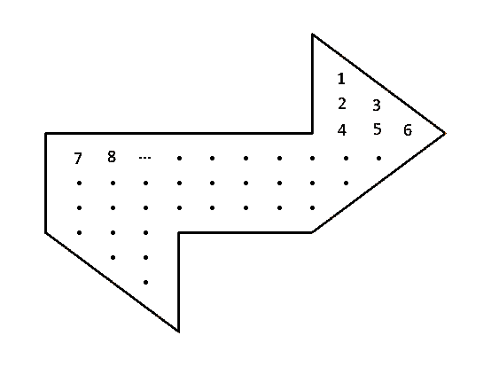
The idea from here is to index this grid and use it as a way to
vectorize functions defined on the region. Then we can define the
discrete Laplacian as a matrix acting on these vectorized functions
and find the eigenvalues of that matrix. There is no correct way to
label the points in our region but its easiest to just name them left
to right, up to down. I wrote a function
index_array which takes binary numpy arrays and gives all
of the ones in the array a unique index. Using the function on a
discrete grid, we get an array that looks like this:
The indexing can go in any order we want. I chose left to right top to
bottom for simplicity.
Now all functions in
can be described by a unique vector in
where is the number of indicies in our grid.
Constructing the Discrete Laplacian
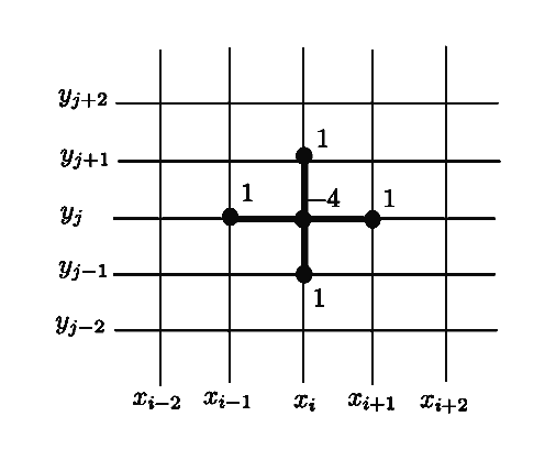
To define an estimate for the Laplacian on this region, we use a
finite difference method. In this case, we use the following 5-point
scheme:
If we want the value of
, we can approximate the second derivatives in both variables by
getting two estimates of the slope with adjacent points and using
those to get an estimate of the second derivative. This works out to
be
where is the distance between adjacent points.
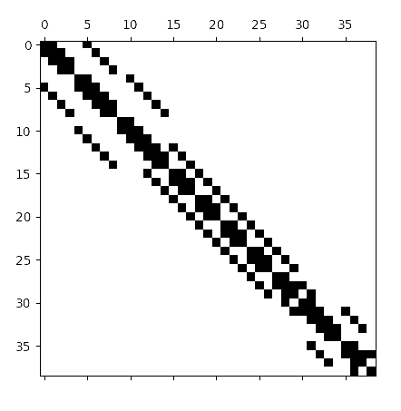
Since our function is described by some vector, we can describe this
transformation as a matrix with the diagonal consisting of -4's and
minor diagonals with 1's depending on how we indexed the region. These
matrices are sparse, so we can use eigsh from
scipy.sparse.linalg to quickly get the eigenvalues and
eigenvectors.
An example of a finite difference laplacian
At this point, we are able to approximately compute the spectra of the
two regions that were claimed to be isospectral and see that they are
nearly identical when we use a high number of points! I encourage you
to get the code from the resources and try this yourself.
Initial Conditions and Animations
There is a bit more we can do now too though. Since we also get the
eigenvectors of the matrix (really vectorized eigenfunctions) and we
know that they form a basis for the space our solutions lie in, we are
able to construct explicit solutions when given some initial
conditions. To best simulate reality, I assumed
and
where is some gaussian which represents
hitting the drum with some initial velocity at a particular point.
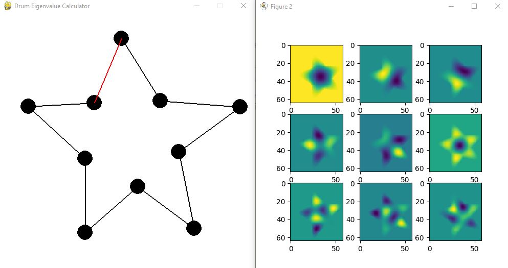
The first few eigenfunctions of a star-shaped drum.
With an explicit solution in time, we can start to make some pretty
simulations for any region we want!
A simulation of a star-shaped drum being hit in one of the corners.
To wrap up, I will mention a few things that could use improvement.
This finite difference method may have some issues with certain drum
shapes. If you imagine a drum which has some long tentacles or other
boundary types, the grid may not be fine enough to capture and
simulate those details. Other than this though, I think it may be
interesting to try and expand this simulation to include the sound the
drum might produce. I tried this a bit but couldn't quite get it to
sound realistic.
Feel free to try this yourself! I made a little interface that allows
you to draw any shape you would like. The spacebar with add points,
the mouse will drag them around, pressing '/' will calculate the
eigenfunctions, and pressing '0' will make the animation! Thanks for
reading!
Resources